Statistical Analysis of Window Impacts on Cooling and Heating Energy Use in Single Family Residence Based on Climate Regions in U.S.A.
@ 2018 KIEAE Journal
Abstract
Window area, location, and selection of glazing are a very important factor in reducing cooling and heating energy use of a building. The primary goal of this research is to investigate the effects of window design variables on annual cooling and heating energy use in a single residence based on climate regions in the United States using statistical analysis.
The methodologies used in this paper are building energy simulations, descriptive statistics, t-test, Latin Hypercube Sampling, and sensitivity analysis. Two groups of window variables are defined and simulated to explore the difference of the simulation results using Latin Hypercube Sampling and t-test. Then, the enter method as a regression model is used to investigate which group of data better predicted annual cooling and heating energy use. Lastly, Standard Regression Coefficients (SRCs) sensitivity indicator is used to determine if the influence of window parameters on cooling and heating energy use varies by different climate zone.
T-test results show that the differences in simulation results between the two groups are not statistically significant. That means that simulations using less number of variables (Group B) can have similar accuracy than simulation with higher number of window variables (Group A). As a result of the regression models, average adjusted R2 is 0.886 for Group A and 0.933 for Group B. Therefore, the regression model using Group B is selected to determine the effect of each variable on energy use. According to SRCs from regression, the most sensitive design parameters for cooling energy use are SHGC, west and south facing windows, while U-value, north and west facing windows are the most sensitive window parameters for heating energy use.
Keywords:
Glazing Thermal Properties, Window to Wall Ratio, Cooling and Heating Energy, Statistical Analysis키워드:
유리창 열적특성, 창면적비, 냉난방 에너지, 통계분석1. Introduction
Most of glazing systems in a building are made of highly conductive materials, so they are particularly prone to large heat gains and losses in buildings because of direct heat gain from solar radiation and heat transfer between outside and inside. It indicates that properly designed window is one of the important factors for an energy efficient building [1].
The International Energy Conservation Code (IECC) was created by the International Code Council in 2000. This code has been adopted by many US state and local governments to establish minimum design and construction requirements for energy efficiency.
In addition, IECC and ASHRAE (United States Heating, Refrigeration, Air Conditioning Engineers Association) define climate regions based on heating degree days, average temperature, precipitation to help builders to identify appropriate climate regions they build. So builders can decide the climate-specific construction guidelines from the IECC they should use.
The primary goal of this research is to investigate the effects of window design variables on annual cooling and heating energy in a single residence based on IECC requirements and different climate regions in the United States using the statistical analysis, which can provide references for window design.
2. Literature Review
According to Moorjani and Asadi [2], one of the most effective ways to reduce energy loss through the building envelope is to optimize thermal performance, area, and placement of the transparent parts of the building. Therefore, architects and general contractors should consider effective way of selecting and placing windows to control solar gains to reduce cooling energy use during the summer season, while reducing thermal losses during the winter season [3].
Although energy simulation can be useful in investigating heat gain or loss through windows, it requires significant time, resources, and technical expertise. In addition, building energy performance evaluation using the simulation tools is usually limited to complex buildings and applied in the later stages of design. For small building such as residences and low-rise apartment buildings, general contractors tend to use personal experience to make design decisions using the minimum requirements specified in the building code [4].
Janelle et al. [5] studied a new modeling approach to quantify building energy performance in the early design stage using multivariate linear regression model based on 27 building parameters for office buildings. This study suggested that the linear regression model can be the basis for effective decision support tools instead of energy simulation at the initial design stage.
One study also proposed to provide architects or general contractors with useful guidelines of the building design parameters to help them select building materials to construct an energy-efficient house [6].
3. Methods
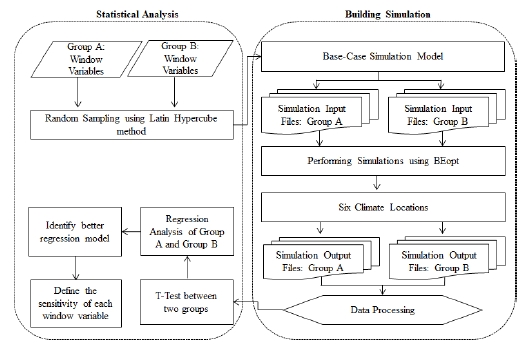
The methodologies used in this research are building energy simulations, descriptive statistics, t-test, Latin Hypercube Sampling (LHS), and sensitivity analysis including multivariate linear regression which determines the impacts of window design variables to building energy use. Fig. 1. shows the flowchart of the overall research methodology.
Two specific questions to be answered through this study are as follows.
1) Is it possible to maintain or improve the predicted simulation results while minimizing the number of design variables?
The number of design variables for considerations should be minimized to provide simple and practical guideline for architects and general contractors. In order to select the efficient window design variables, two groups of window variables are defined in Table 1.
As seen in Table 1., twelve parameters are considered as window variables for Group A that were used in the previous research [6], and six parameters are used for Group B as an alternative. Since simulations of each group require extensive input for sensitivity analysis, Latin Hypercube Sampling (LHS) is used to develop the combinations of the window variables within the specified ranges for comprehensive simulation input files for sensitivity analysis. According to Dominguez-Munoz [7] et al., Latin Hypercube Sampling (LHS) is a common sampling technique for building energy simulations for a minimum number of simulations because each parameter has uniform distributions since all values within the specified range are considered equally probable design variables.
After performing simulations using a input variable from LHS, t-test was performed to investigate the difference between the results of two simulation groups. If the difference of simulation results between the two groups is not statistically significant (at 95% confidence level), it means that even with a small number of variables, it is possible to achieve the similar results with many variables. In addition, the comparison of regression results from two groups has been conducted to identify which group of regression model explains the simulation results better.
2) Does the window design variables have different effects on energy usage depending on climate conditions (climate regions)?
Because the cooling and heating energy demand is sensitive to different climate zones, simulations are conducted in six climate zones defined by ASHRAE [8]. Six climates are selected to explore the impact of local weather conditions, and they represent the average weather conditions of very-cold (Minneapolis, MN); cold (Chicago, IL); mixed-humid (Atlanta, GA); hot-humid (Houston, TX); hot-dry (Phoenix, AZ); and marine (Los Angeles, CA) climates [9]. TMY3 weather data for each selected location were used for the simulations. The summary of the climate characteristics is shown in Table 2.
3.1. Statistical Analysis
Sensitivity analysis is a study of the influence of independent variables on dependent variable in certain condition [10]. Therefore, sensitivity analysis has been used to study the effects of window design variables such as WWR, orientation and thermal properties of glazing on energy usage. There are two main approaches of sensitivity analysis: local sensitivity analysis and global sensitivity analysis. Local sensitivity analysis investigates the impact of one variable as keeping others fixed, while global sensitivity analysis uses all variables to investigate the relative impacts [6,11,12]. For this research, global sensitivity analysis has been used to study the impacts of all design parameters simultaneously on energy consumption.
In sensitivity analysis, regression is the most widely used method of building energy analysis because it is fast to compute and the results are easy to understand. From the regression model, many indicators can be used for the sensitivity indices such as SRC (Standard Regression Coefficients), PCC (Partial Correlation Coefficients), and their rank transformation (SRRC standardized rank regression coefficient), and partial rank correlation coefficient (PRCC) [13]. One study has applied SRC indicator to determine the main variables affecting the maximum cooling load of a perimeter zone in a three-story office in southern Spain [14].
For this research, SRC sensitivity indicator is also used to study the influence of window parameters on cooling and heating energy use in different climate zones.
3.2. Base-case Simulation Model
Base-case simulation model is a single-family residence based on U.S. Census Beaureu and IECC requirements of wall, floor, and roof assembly, and HVAC system efficiency specifically for single-family residence.
A 232 m2 (2,500 ft2) single-family residence is considered as the basis for this study based on U.S. Census Beaureu [15]. The base-case house is assumed to have light-weight wood-frame construction with 5 cm x 10 cm (2 inches x 4 inches) wall studs spaced at 40.6 cm (16 inches) on-center and 5 cm x 15 cm (2 inches x 6 inches) ceiling joists/roof rafters spaced at 61 cm (24 inches) on-center, a 10 cm (4-inch) slab-on-grade floor, and an unconditioned-vented attic space. The base-case house has the 2015 IECC5) specified climate-specific exterior wall assembly (3.52 m2·°C/w (R-20)) and ceiling assembly (8.63 m2·°C/w (R-49)), slab perimeter insulation (0.61 m (2 ft) 1.76 m2·°C/w (R-10) perimeter with 0.88 m2·°C/w (R-5) gap). The base-case HVAC system includes a SEER6) 13 central air-conditioner with a 78% AFUE7) furnace conforming to the 2015 IECC. The heating and cooling set-points are 21.7°C (71 ºF) for the winter and 24.4°C (76 ºF) for the summer without setback temperature.
For the simulation, BEopt simulation program ver. 2.7 was used. BEopt stands for Building Energy Optimization, and has been developed by the National Renewable Energy Laboratory (NREL) in support of the U. S. Department of Energy (DOE). BEopt software is specially developed for building energy simulation of residence to utilize EnergyPlus simulation engine, and provides detailed simulation analysis to evaluate residential building energy consumptions [16].
4. Findings
The results of this study include the follows: 1) simulation results of base case house in six selected locations, 2) t-test results between Group A and Group B as explained in Table 1., 3) comparison of regression models between Group A and Group B, and 4) SRC (Standard Regression Coefficients) results of a selected regression model.
4.1. Base-case Energy Use
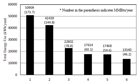
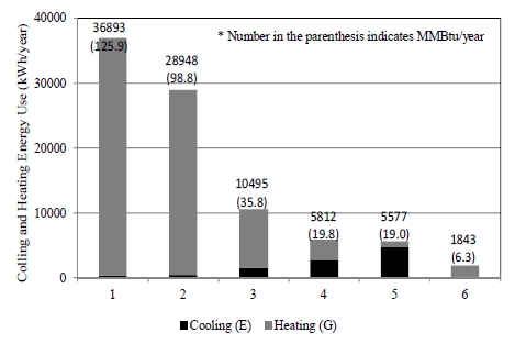
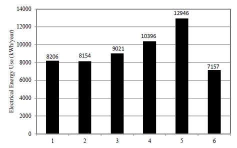
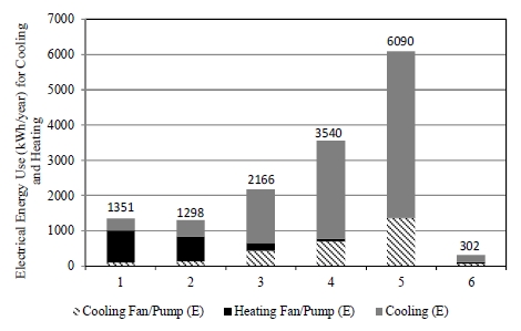
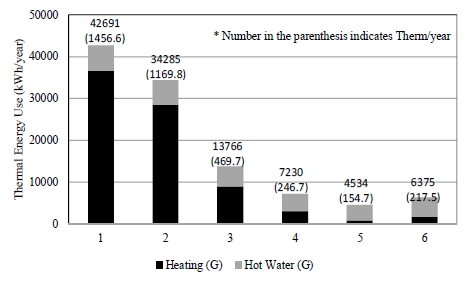
From the BEopt output, the thermal energy use and electricity use are investigated on an annual basis. Fig. 2. to Fig. 6. show the annual total energy use, electricity use and thermal energy use for the six selected locations including: 1) Minneapolis, MN, 2) Chicago, IL, 3) Atlanta, GA, 4) Houston, TX, 5) Phoenix, AZ, and 6) Los Angeles, CA. Table 3. indicates the case number in X axis in Figures from 2. to 6.
Fig. 2. shows total energy use for a year (kWh/year) including cooling and heating, fan, lighting, and other appliances. Fig. 3. excludes the energy use of lighting and other appliances from Fig. 2. and shows only cooling and heating energy use since energy uses of lighting and other appliances show the same in each region.
Fig. 4. shows electrical energy use including cooling, fan, lighting, and other appliances, and Fig. 5. shows only cooling and fan energy for heating and cooling from electrical energy use.
Lastly, Fig. 6. shows thermal energy use including heating and domestic hot water energy use.
More energy use for heating was observed specially in Minnesota and Illinois, and more energy usage for cooling was observed specially in Arizona and Texas, which conform to the heating degree days and cooling degree days (Table 2.). These variations in cooling and heating energy are a direct indication of the local climate features such as long winter period of Minnesota and Illinois and long summer period of Arizona and Texas. The relatively mild climate condition in California and Georgia shows that cooling and heating energy use has been used relatively less than other regions. In addition, lighting and other appliances show a large share of electrical energy use.
4.2. Statistical Results
Independent two-sample t-test was conducted to explore the difference in the means of the simulation results from Group A which used 12 window variables and Group B which used 6 window variables. The sample size of Group A and Group B is 120 (n=120) and 80 (n=80), respectively. The sample size was determined as recommended by Latin Hypercube Sampling method which uses 10 times the number of variables [17].
For statistical analysis, the null hypothesis is that there is no difference between the means of two simulation groups. Table 4. shows the results of t-test for annual cooling and heating energy use. As shown in Table 4., the difference in annual cooling and heating energy use between the two groups is not statistically significant at 95% confidence level. Therefore, the null hypothesis fails to be rejected because the p-value is larger than 0.05. This results mean that even though the simulations are performed using less number of window variables, it can have similar accuracy to simulations using higher number of window variables.
Regression analysis is also performed to investigate which group of data better predicts annual cooling and annual heating energy use. For the regression model, the enter method was used, which all independent variables are simultaneously entered into the regression model. This method is an appropriate method for analyzing the small numbers of independent variables or when the researcher does not know which independent variables can yield the best regression equation [18].
Since this research investigates the effect of all the variables used in this study and the number of variables is relatively small, the enter method was considered appropriate for the multivariate regression modeling. Table 5. shows the adjusted R2 which indicates how closely data such as WWRs, SHGC and U-value can explain annual cooling and annual heating energy use. It was found that the overall regression models show a good fit. The multiple linear regression in each location yields an adjusted R2 from 0.932 to 0.960 in Group A and from 0.918 and 0.966 in Group B for annual cooling energy. The regression for annual heating energy yields an adjusted R2 from 0.798 to 0.838 in Group A and from 0.896 to 0.944 in Group B. The average adjusted R2 for both cooling and heating energy is 0.886 for Group A and 0.933 for Group B. Therefore, the regression model using Group B is selected to investigate the effect of each variable on energy use. In addition, the value of Durbin-Watson in all regression models is close to 2, which means that there is no auto-correlation between data.
Tables 6. and 7. describe the influence of each variable on annual cooling and annual heating energy use in six different locations.
Standardized Regression Coefficient (SRC) is used to represent relative contributions of each variable to annual cooling and heating energy variability in each region. T- and p-value are also presented to check statistically significance of each variable.
5. Discussions
5.1. Window Design Variables for Cooling Energy
It was found that window design variable that has the most important effect on cooling energy usage is SHGC which is consistent across all locations according to the SRC in Table 6. For example, California shows the highest sensitivity to SHGC followed closely by Illinois. On the other hand, the U-value of the window is not statistically significant (p>0.05) in relatively cold regions such as Minnesota and Illinois. U-value in relatively hot climate zone such as Texas and Arizona is statistically significant (p<0.05), but it has less impact on the annual cooling energy use than other variables. Therefore, in Texas and Arizona where the cooling load is relatively high, SHGC is more important than the U-value in window selection. Not surprisingly, it has been found that as WWR increases, the cooling energy consumption increases. The SRCs were also observed to determine which orientation of WWR has more influence on cooling energy consumption. It is found that WWR in the west and east has a greater effect on the use of cooling energy than the north and south. This is due to excessive amount of solar radiation at low angle coming from the east and west sides in the morning and afternoon during summer. Therefore, it is appropriate to select a low SGHC window with a smaller window area in the east and west sides specially in hot climate zone (cooling dominated region) in order to reduce cooling energy.
5.2. Window Design Variables for Heating Energy
As shown in Table 7., it was found that U-value is the most influential on the amount of heating energy usage. Furthermore, both SHGC and U-value are statistically significant (p<0.05), and these two variables affect the heating energy demands more than other WWRs. This results show different patterns from the results of cooling energy use. For cold climate zones (heating dominated region) such as Minneapolis and Illinois, high SHGC and low U-value should be considered more than other variables to reduce the heating energy demands.

Standardized Regression Coefficient (SRC) of each variable for annual heating energy use in six locations.
For WWR, window areas in the north and west are more influential to the heating energy use than other orientations. It is because there is less opportunity to receive solar radiation than other orientations of windows while there is more conduction heat loss due to large window areas at the same time. This results in more heating energy consumption because of large window areas in the north and west sides. It is also found that WWRs on the south side is not statistically significant (p>0.05) for all locations. For the window layout, consideration of WWR of the north, west and east is more important than that of the south to reduce the heating energy use.
6. Conclusion
Building simulation can accurately predict building energy use, but it is difficult to be utilized by architects and general contractors because it requires higher level of engineering expertise. The purpose of this study is to present the data that can be referenced by the architects and general contractors that investigates the effect of window properties including SHGC and U-value, and WWRs on the energy consumptions in six climate regions representing the United States.
In order to obtain the data for the statistical analysis, the extensive numbers of simulations using the average size of the residence in the U.S. were performed with BEopt simulation program. For simulations, two groups with different numbers of window variables were used.
To study the optimum numbers of window variables, t-test was performed using the results from two groups.
T-test results show that the difference in simulations results between the two groups are not statistically significant. Then, a regression model of two groups is developed to identify a better fit to the simulation results. All adjusted R2 values obtained from the multivariate regressions show a good fit to the simulation results. However, the average adjusted R2 is 0.886 for Group A and 0.933 for Group B, so standardized regression coefficients (SRCs) generated in Group B are used for sensitivity analysis. This results suggest that the regression model can be developed using a reduced numbers of variables, and also can be useful for the architect and general contractor for window design considerations.
According to SRCs from the regression, the most sensitive design parameters for cooling energy use are SHGC and west and south facing windows, while U-value and north and west facing windows are the most sensitive window parameters for heating energy use.
The results of this research considered the relative importance of window design variables based on different climate regions for single family residence, and have limitations for builders to apply to have window designs specifically. Future ongoing research needs to perform in-depth analysis to provide detailed range of appropriate window thermal properties varying window area and construction costs based on climate regions. This combination of results can provide builders with guideline to consider better window design decisions.
References
-
Samar, J, Salman, A, Thermal and economic windows design for different climate zones, Energy and Buildings, (2011), 43, p3208-3215.
[https://doi.org/10.1016/j.enbuild.2011.08.019]

- Vahid, M, Somayeh, A, Assessing the effects of glazing type on optimum dimension of windows in office buildings, 50th ASC Annual International Conference Proceedings, (2014, Oct).
-
Andrea, G, Giovanni, P, Francesca, C, Piercarlo, R, Paolo, B, Analysis and modelling of window and glazing systems energy performance for a well insulated residential building, Energy and Buildings, (2011), 43, p1030-1037.
[https://doi.org/10.1016/j.enbuild.2010.12.032]

-
Mora, R, Bedard, C, Rivard, H, A geometric modelling framework for conceptual structural design from early digital architectural models, Advanced Engineering Informatics, (2008), 22, p254-70.
[https://doi.org/10.1016/j.aei.2007.03.003]

-
Janelle, H, Joseph, D, David, H, Ranji, R, Multivariate regression as an energy assessment tool in early building design, Building and Environment, (2012), 57, p165-175.
[https://doi.org/10.1016/j.buildenv.2012.04.021]

-
Yusuf, Y, Koray, K, Türkan, G, Zeynep, A, An approach for developing sensitive design parameter guidelines to reduce the energy requirements of low-rise apartment buildings, Applied Energy, (2012), 93, p337-347.
[https://doi.org/10.1016/j.apenergy.2011.12.048]

-
Dominguez-Munoz, F, Cejudo-Lopez, MJ, Carrillo-Andres, A, Uncertainty in peak cooling load calculations, Energy Build, (2010), 42, p1010-8.
[https://doi.org/10.1016/j.enbuild.2010.01.013]

- ASHRAE, ASHRAE 90.1-2007 Energy standard for buildings except low-Rise residential buildings, Atlanta, GA, American Society of Heating, Refrigeration, and Air-Conditioning Engineers, (2007).
- Mini, M, An analysis of off-grid, off-pipe housing in six U.S. climates, Ph.D. Dissertation, Texas A&M University, (2009).
- Andrea, Saltelli, et al. , Sensitivity Analysis in Practice, John Wiley & Sons, UK, (2004).
-
Heiselberg, P, Brohus, H, Hesselholt, A, Rasmussen, H, Seinre, E, Thomas, S, Application of sensitivity analysis in design of sustainable buildings, Renew Energy, (2009), 34, p2030-6.
[https://doi.org/10.1016/j.renene.2009.02.016]

-
Yıldız, Y, Arsan, DZ, Identification of the building parameters that influence heating and cooling energy loads for apartment buildings in hot-humid climates, Energy, (2011), 36, p4287-96.
[https://doi.org/10.1016/j.energy.2011.04.013]

-
Wei, T, A review of sensitivity analysis methods in building energy analysis, Renewable and Sustainable Energy Reviews, (2013), 20, p411-419.
[https://doi.org/10.1016/j.rser.2012.12.014 ]

-
Ilaria, B, Vincenzoc, C, Analysis of the building energy balance to investigate the effect of thermal insulation in summer conditions, Energy and Buildings, (2012), 52, p168-180.
[https://doi.org/10.1016/j.enbuild.2012.06.004]

- U.S. Census Beaureu, Highlights of Annual 2016 Characteristics of New Housing, Available at https://www.census.gov/construction/chars/highlights.html (accessed Sep 1, 2017) (2016).
- NREL (National Renewable Energy Laboratory), BEopt, Available at https://beopt.nrel.gov/ (accessed Nov 15, 2017) (2017).
- Simlab, Software package for uncertainty and sensitivity analysis. Joint Research Centre of the European Commission, Available at https://ec.europa.eu/jrc/en/samo/simla (accessed Oct 2, 2017) (2017).
- IBM Corp., Released 2011. IBM SPSS Statistics for Windows, Version 20.0, Armonk, NY, IBM Corp.
