Comparison of Sensitivity Analysis Methods for Building Energy Simulations in Early Design Phases: Once-at-a-time (OAT) vs. Variance-based Methods
© Copyright Korea Institute of Ecological Architecture and Environment
Abstract
Sensitivity analysis offers a good guideline for designing energy conscious buildings, which is fitted to a specific building configuration. Sensitivity analysis is, however, still too expensive to be a part of regular design process. The One-at-a-time (OAT) is the most common and simplest sensitivity analysis method. This study aims to propose a reasonable ground that the OAT can be an alternative method for the variance-based method in some early design scenarios, while the variance-based method is known adequate for dealing with nonlinear response and the effect of interactions between input variables, which are most cases in building energy simulations.
A test model representing the early design phase is built in the DOE2 energy simulations. Then sensitivity ranks between the OAT and the Variance-based methods are compared at three U.S. sites.
Parameters in the upper rank by the OAT do not much differ from those by the Main effect index. Considering design practices that designers would chose the most energy saving design option first, this rank similarity between two methods seems to be acceptable in the early design phase.
Keywords:
Sensitivity Analysis, Building Energy Simulation, Once-at- a-time, OAT, Variance based method, Main effect index1. Introduction
It is well known that design decisions made during early building design phase greatly impact on the energy performance of the designed building. For more responsive and reliable decisions, using building energy simulation becomes an industry de-facto standard design process; after initial mass study, designers try to find the most energy saving design options over continuous simulation experiments by various design options. Often selecting model parameters and their design options follow the design guidelines [1]. However, there are no universal priority of energy sensitive parameters; a set of energy sensitive parameters varies upon climate, building type, building shape, range of design alternatives, etc.
Sensitivity analysis offers a good guideline that is fitted to a specific building configuration. Although designers know the merit of sensitivity analysis, they don't have enough time for doing sensitivity analysis in every design situation, as well as only simulation experts trained with statistical background can produce reliable sensitivity analysis. Therefore sensitivity analysis is still too expensive to be a part of regular design process.
2. Sensitivity analysis for building energy simulations
Sensitivity analysis is to identify how different types and degrees of model parameters (i.e., input variables) affect the output responses of simulation model. Also it sets up an order by the strength and relevance of the model parameters in determining the variation of output response. Sensitivity analysis is performed by many reasons when mathematical (simulation) model is initially created or it needs to be refined. Concerning building energy simulation model, purposes of sensitivity analysis include:
- 1) Better understanding of the relationship between model parameters and output responses of the simulation model,
- 2) Testing the model robustness with presence of diverse sources of uncertainty in the model parameter, and
- 3) Selecting model parameters with greater impacts or screening model parameters with least impacts and thus simplifying the simulation model or the scope of considerations.
When a modeler creates a new simulation model, sensitivity analysis is useful by the first two reasons. When a designer uses the created model, sensitivity analysis offers a clue on which model parameters the designer needs to first focus.
Prevalent methods of sensitivity analysis are largely classified into five categories as listed as in Table 1. The first three methods are relatively known and have been often referred in literature concerning sensitivity analysis of building energy model. For local derivative method, however, it is quite hard to approximate building energy models by the Taylor series; the regression (not necessarily linear) appears to be more doable and useful for an alternative of the Taylor series.
When the model response tends to be nonlinear and/or strong correlation between model parameters and model interactions are observed, the first four methods are known resulting in inaccurate sensitivity measure. As this limitation is often the case of building energy models, the Variance-based method, a global sensitivity algorithm, is known better suitable for sensitivity analysis of building energy model.
Basically the variance-based method assumes a full exploration of input variable space accounting for interactions and nonlinear responses, which means theoretically it requires a full factorial analysis. It is a big computational burden as well as a huge effort for the evaluator who prepares input data. Since sensitivity analysis of building energy model is most useful at early design phases when a majority of design information is still undecided or not known, evaluators encounter a practical barrier against continuing sensitivity analysis due to a difficulty of data collection and preparation. Although the Variance-based method is known performing better than the first four methods, therefore, in some cases evaluators choose the most simple algorithm such as the OAT (Once-at-a-time) because it could be only available solution for them.
Initiated by this practice often observed in the field, this study aims to propose a reasonable ground that the OAT (the simplest) can be an alternative method for the Variance-based method (the most complex) in some sensitivity analysis scenarios by means of comparing results by the two in the context of practical design case.
3. OAT method
As its name indicates, the model response is measured for each change of each model parameter while the other parameters keep hold, i.e., there is no simultaneous change of multiple parameters, thus no detection of the presence of interactions between input. The OAT typically proceeds as follows:
- Step 1: Change the value of a model parameter from its base value while keeping the others at their base value.
- Step 2: When exploring the space of the first model parameter is complete, it is set to its base value back. And then repeat for each of the other model parameters in the same manner.
- Step 3: Calculate the degree of model response displacement by each model parameter (Equation 1) and then compare the magnitude for all the evaluated model parameters using plots.
(Eq.1)
where the model is a function Y = f(Xo, X1, …, Xn), and X0 indicates the vector of base values for X.
Since moving one value of model parameter at a time saves a lot of computational effort and also gives very intrinsic perception of “how it goes” to the evaluator, the OAT is often preferred by evaluators because of its high practicality.
In many cases of sensitivity analysis of building energy model in the design context, values of model parameters tend to be discrete. For instance, U-value of single pane of window glazing does not always smoothly vary when the glazing pane becomes double. From time to time this discrete feature as well as a limited knowledge about value of model parameters in the early design phase makes the exhausted exploration over all the input variables harder. To perform a global sensitivity analysis, therefore, strong simulation expertise and experience in data preparation for compensating this discrete feature are required. In this case practitioners tend to (or are forced to) choose the OAT, rather than the global sensitivity analysis, despite its comprehensive merits.
4. Variance-based method
The Variance-based method measures sensitivity across the whole input space dealing with nonlinear response, and the effect of interactions between input variables, thus it is a global sensitivity analysis; the “sensitivity” is calculated by the normalized variance of the model response for a specific input variable and “effect” is calculated by decomposing the variance into fractions which can be attributed to inputs or a certain set of inputs.
Decomposing the variance assumes the model is a function Y = f(X), where X is a set of input variables {X1, X2, …, Xn} and Y is the model response. Also the inputs are assumed to be independent and uniformly distributed within the input space, which is to ensure the generality. Then f(X) can be decomposed such as:
| (Eq.2) |
where f0 is a constant, fi is a function of Xi, and fij is a function of Xi and Xj.
Equation 2 enables the following functional decompositions with respect to the conditional expected value for each Xi.
| (Eq.3) |
| (Eq.4) |
| (Eq.5) |
Along with Equation 3 to 5, the following decomposition of variance is also enabled.
| (Eq.6) |
| (Eq.7) |
| (Eq.8) |
where X~i indicates the set of varying all the input variables except Xi.
Eventually Equation 6 demonstrates how the variance of the model response can be decomposed into the terms with respect to each input variable Xi (the first parenthesis) as well as the interaction between input variables (the second parenthesis). It also demonstrates how much Xi contributes “alone” to the total variance of the model output and how much Xi and its interactions with other input variables contributes to the total variance of the model output. The former is called the Main effect index and the latter is called the Total effect index of Xi. Both indexes are typically standardized by dividing by the total variance, i.e., Var(Y).
5. Comparison of the OAT and the Main effect index
While the OAT could be the simplest method of sensitivity analysis, the Variance-based method requires a quite large effort for data preparation and computational expense. This study aims at finding out an opportunity that the OAT can be used alternatively in some design situations such as early design phases. For this experiment, the test set is configured as follows.
5.1. Test configuration
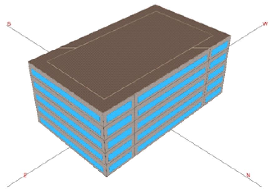
An ideal five story office building with 1500 m2 (50m x 30m) of each floor area is selected for simulations as depicted as in Figure 1. Initially the 50m long side is set to face the South (thus the other side faces the North). It is a regular office operating from 8am to 5pm weekday. It is built in the DOE2 building energy simulation via Autodesk Green Building Studio [4]; the base value includes 40% of the window-wall ratio, R15 roof deck, R13+3.8 metal frame exterior wall, double clear U-SI 0.56, SHGC 0.69, VLT 0.78 window glazing, VAV (Variable Air Volume) with COP 5.0 chiller, 82% gas boiler and VSD (Variable Speed Drive) fans, and no lighting controls. Also its built environment includes 300 occupants, 9.69 W/m2 of LPD (Lighting Power Density), 14.42 W/m2 of EPD (Electric Power Density), and 0.4 ACH of infiltration for perimeter zones.
Additionally to observe sensitivity variations depending on locations, three sites - Miami, FL, San Francisco, CA, and Chicago, IL, which represent the ASHRAE climate zone 1, 3, and 5, respectively - are chosen.
5.2. Comparison of the OAT and Main effect indices
Model parameters that are known as “building energy contributors” and typically being decided in the pre-schematic and schematic design phase are selected, and also their design options considering actual industry practices in the U.S. are chosen. These parameters and options are listed in Table 2.
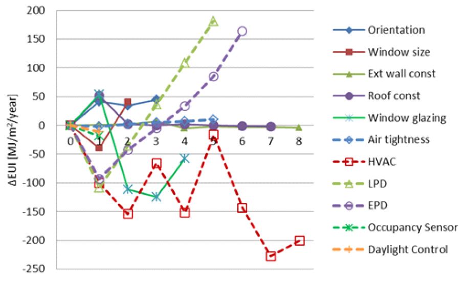
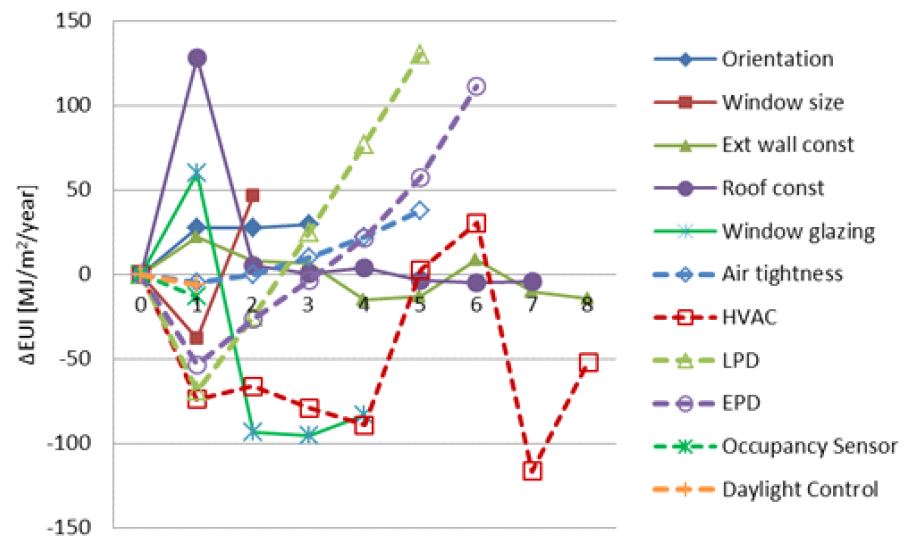
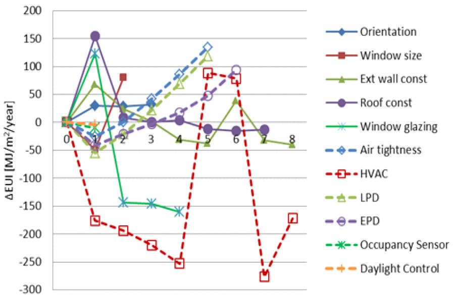
With the EUIs calcuated using the base model and its variants in Table 2, the delta EUIs, i.e., the difference between the base EUI and the alternative EUI, for three site cases are calculated and depicted in Figure 2, 3, and 4. The x axis of charts indicates the design option label for each model parameter (Table 2) while “0” indicates the delta EUIs of the base model is zero.
Only the Main effect index for each model parameter is considered for this time. Since a full factorial analysis requires practically impossible simulation runs (4x3x9x8x5x7x9x6x7x2x2), the Latin hypercube sampling [5] is employed. Sensitivity ranks by the Main effect index for each model parameter are shown in Table 3 and then compared to the OAT ranks.
In Table 3, it is observed that parameters in the upper rank (from 1st to 5th) by the OAT do not much differ from those by the Main effect index. As expected, reducing both internal and external heat gains seems to be the most urgent design action in hot climate (represented by Miami, FL). HVAC performance and reducing heat loss seems to be the most urgent design action in cold climate (represented by Chicago, IL). For San Francisco, CA with mild winter, thus almost no heating required, reducing both internal and external heat gains seems to be the most urgent to reduce cooling energy of an office building in summer.
Considering the design practice that designers would choose the most energy saving design option first and/or would more concern the most energy sensitive design parameter, this rank similarity between two sensitivity analysis methods seems to be acceptable in the early design phase.
6. Discussion and Conclusion
This paper presents a pilot study to demonstrate the OAT can be an alternative for the Variance-based method in the early design phase. As the study is still in its initial stage, some limitations still need to be mentioned;
1) The Total Effect index that takes into account of a serious interaction between model parameters need to be tested against the OAT,
2) More complex base model and/or more design options varying upon design context need to be tested. In particular, the range of design options should be extended as well as the design options resulting in more discrete input value variation should be heavily tested, and
3) Other Variance-based methods such as Metamodeling [6] and FAST (Fourier Amplitude Sensitivity Test) [3] need to be tested.
Sensitivity analysis is a useful tool in making design decisions for energy conscious building design; it produces configuration-specific ranks of design variables than design guidelines, such that designers can more focus on a smaller number of design variables. Unfortunately it is still difficult for most building design practitioners and also still expensive in terms of computation cost and analysis expertise. If a simpler and cheaper method such as the OAT would not seriously distort the result by more accurate, but more expensive sensitivity analysis methods, suggesting usecases and scenarios for this alternative method would enhance the productivity of design practitioners.
Announcement
This study was supported by the Research Program funded by the Seoul National University of Science and Technology.
References
- ASHRAE Advanced Energy Design Guides, ASHRAE, https://www.ashrae.org/standards-research--technology/advanced-energy-design-guides.
-
Morris, M. D., (1991), Factorial sampling plans for preliminary computational experiments, Technometrics, 33, p161-174.
[https://doi.org/10.1080/00401706.1991.10484804]

- Saltelli, A., K. Chan, and M. Scott (Eds.), (2000), Sensitivity Analysis. Wiley Series in Probability and Statistics, New York, John Wiley and Sons.
- Autodesk Green Building Stuido, Autodesk, http://gbs.autodesk.com.
- Iman, R.L., Davenport, J.M., and Zeigler, D.K., (1980), Latin hypercube sampling (program user's guide).
-
Storlie, C.B., Swiler, L.P., Helton, J.C., and Sallaberry, C.J., (2009), Implementation and evaluation of nonparametric regression procedures for sensitivity analysis of computationally demanding models, Reliability Engineering & System Safety, 94(11), p1735-1763.
[https://doi.org/10.1016/j.ress.2009.05.007]


