The audit method of cooling energy performance in office building using the Simple Linear Regression Analysis Model
ⓒ Copyright Korea Institute of Ecological Architecture and Environment
Abstract
In order to upgrade the energy performance of existing building, energy audit stage should be implemented first because it is useful method to find where the problems occur and know how much time and cost consumption for retrofit. In overseas researches, three levels of audit is proposed whereas there are no standards for audit in Korea. Besides, most studies use dynamic simulation in detail like audit level 3 even though the level 2 can save time and cost than level 3. Thus, this paper focused on audit level 2 and proposed the audit method with the simple linear regression analysis model.
Two parameters were considered for the simple regression analysis, which were the monthly electric use and the mean outdoor temperature data. The former is a dependent variable and the latter is a independent variable, and the building’s energy performance profile was estimated from the regression analysis method. In this analysis, we found the abnormal point in cooling season and the more detailed analysis were conducted about the three heat source equipments.
Comparing with real and predicted models, the total consumption of predicted model was higher than real value as 23,608 kWh but it was the results that was reflected the compulsory control in 2013. Consequently, it was analyzed that the revised model could save the cooling energy as well as reduce peak electric use than before.
Keywords:
Simple Linear Regression Analysis, Energy Performance Audit, Office Building1. Preface
1.1. Background & Purpose of This Study
The government recently established the first basic plan for constructing green buildings in order to reduce green gas which is generated from buildings by 26.9% compared to BAU (Business As Usual) until 2020.
Since the importance of energy performance improvement for the existing buildings rather than new ones gets bigger as a country becomes an advanced one, the Korean government has planned to improve the energy performance of the existing buildings through the application of ‘Energy Performance Improvement Standards for Existing Buildings’ from the first half of 2015. This is an effort to improve the energy performance or efficiency as a green remodeling project for reducing the cooling/heating loads and energy consumption of the existing buildings and especially it is intended to encourage the expansion of green buildings to the private area after applying it for the public area first.
However, for the domestic green remodeling projects which have been implemented as pilot projects in the public area since 2013 in order to expand the green buildings and to establish the guidelines on green remodeling, the performance improvement of the building envelopes has been induced by subsidizing for the construction costs in the areas related to the building envelop systems preferentially such as the insulation of walls, the replacement of windows and doors and the airtightness performance improvement, etc. In addition, it is intended to improve the performance through some supporting services such as the evaluation of the status of aged buildings (Green Clinic) and the design consulting (Green Coach), etc., in order to enhance the performance of the projects. However, it is in the situation that there are insufficient specific studies for diagnosing the energy use status of buildings quantitatively and for establishing the realizable strategies. And especially, since it is somewhat hard to get some detailed information on the buildings from most of the existing buildings, it is important to closely audit such buildings by using various kinds of equipment or simulations, but also it is very important to audit the energy performance of the target buildings and the problems while being used by using only some kinds of essential information.
Thus, in this study, it is intended to suggest some methods for diagnosing the energy performance of buildings by using some relatively simple and economic statistical approaching methods compared to some simulation methods only with some kinds of information which was collected for enhancing the effects of the green remodeling projects that have been implemented by the government until now and also is intended to provide with some basic information for establishing the guidelines for diagnosing when implementing the green remodeling projects for the existing buildings by analyzing the effects.
1.2. Methodology and Scope of This Study
According to the existing studies, it was found that the effects were big only when implementing the energy performance improvement projects centered on the relevant buildings in the size, 500~10,000m2. Furthermore, according to ‘Advanced Energy Retrofit Guide for Office Building’ as a foreign energy performance improvement guideline, the audit levels can be chosen from Level 1 to 3 depending on the economic conditions of the building owners when deciding the audit level for the target buildings and the costs to be used for and scope of each level are shown in Fig. 1. In addition, for ASHRRAE Standards, the audit levels are divided into 4 ones in order to improve the energy performance improvement of buildings. And the goals and scopes of each level are shown in Table 1. Especially, the scope of conducting a real audit is divided into Level 1 to 3. And as the level goes up, the works done in the previous levels in common are also done. And since the approaching methods can be different by a little depending on the characteristics of buildings, the level 2 and 3 are not distinguished clearly.
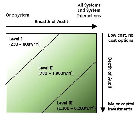
The range of audit costs are estimated based on market research and previous estimates by the California Energy Commission (2000)
However, unlike the foreign cases mentioned above, it is in the situation that the standards or guidelines on the audits are incomplete in Korea yet. Moreover, in many domestic studies, there are used some strategies for improving the energy performance through some calibration works between the simulations and the real consumption of energy by using some dynamic simulations such as 'Energy Plus' as the level 3. Such a method has a strength that the accuracy is high, but a weakness that much time and cost must be spent for realizing almost the same simulations as the target buildings.
Therefore, in this study, it is intended to follow the following process in order to analyze the effects of the diagnosing methods quantitatively from the operational aspect at level 2 for establishing the guidelines on the domestic green remodeling audits.
- (1)Figure out the characteristics of a simple linear regression analysis method which is relatively simpler compared to the simulation methods.
- (2)Analyze the energy consumption status of the target buildings and the energy performance profiles by applying the simple linear regression analysis method after selecting the relevant office buildings targeted for green remodeling.
- (3)Analyze the effects by comparing the actually measured data and the calibrated data after deducting and improving the problems through the audits.
2. Simple Linear Regression Analysis Method
The methods for calculating and modeling the energy consumption of buildings can be broadly divided into two approaches, that is, a Forward (Classical) Approach and a Data-driven (Inverse) Approach. The former is a method for estimating the results based on the given information and it is idealistic when designing a building or a system. On the other hand, the latter is a method for deciding the mathematical explanations on the system and the parameters of the system under the situation that the input values and the output ones are known. It can be said that a Simple Linear Regression Analysis Model is a method belonging to the latter. And it can be said that the model is more appropriate method when retrofitting the completed buildings by statistically analyzing the correlation with the various kinds of variables such as energy consumption which is calculated and measured at the steady state and climates and the schedule of a person in a room. In 2002, ASHRAE suggested an Inverse Model Toolkit (IMT) in order to evaluate the energy reduction quantity of buildings based on the actual consumption by enhancing the method, PRISM (Princeton Scorekeeping Method) which was developed for housing as such a regression method in eary 1980's. The model became applicable even for commercial buildings after subdividing a model having 5 parameters by using the outside temperature as an independent variable and the energy consumption as a dependent variable.
Especially, such a method indicates the degree of correlation by using the coefficient of determination(R2) as the correlation between the independent and dependent variables. The method has a strength that can predict the future values depending on the changes in independent variables after deducting a prediction equation by using such a correlation. In addition, such a method is a kind of empirical one. And since it is relatively simple, it can be used in various situations. So, it is used most widely and also is useful in finding out some strategies with which can save some energy from the actual buildings.
3. Case Analysis
3.1. Selection of Target Buildings & Information Gathering
The target buildings for green remodeling are the ones which more than 15 years have passed after obtaining the use approval certificate and have bigger than 3,000m2 of gross floor area. Thus, in this study, the G research building of the K Research Institute which is located in Daejeon Metropolitan City was selected as the target building. The information on the target building which was obtained through a pre-site work is shown in Table 2.
For the target building, more than 100 kinds of eco-friendly technology such as the double envelops on the southern side when it was designed, the natural lighting using the atrium and the solar control louver, etc., were applied. In addition, the metering system was established as a part of the energy performance improvement project during summer in 2011 and the information on the gas & electricity consumptions are sent in real time from 47 station points (45 for electricity and 2 for gas) by using BAS(Building Automation System) and AMI (Advanced Metering Infrastructure).
And since the occupants and the indoor devices in G-building have increased compared to the time when the building was designed, the AHU no. 1 &2 were replaced with EHP-type AHUs in order to respond to the cooling/heating loads accordingly. Therefore, in this building, three AHUs except for the one (Direct Expansion AHU; AHU-4) which is dedicated to the conference hall are mainly operated, and the AHU-1 &2 for the main living room are operated together with the EHP.
In addition, the HVAC type of G-building is a VAV(variable air volume)- type. And the building which is cooled with 2 screw chillers (during day and night) and the ice storage system are operated in parallel. And in case of heating, the convector system which is connected to the steam boiler is operated via the AHU. However, this building as a public building has the characteristics that the compulsory operation is influenced in accordance with the government directions when operating the cooling & heating systems unlike the general office building by adjusting the temperature down to 27~28℃ when cooling, 19~18℃ when heating, 60 days to 42 days as the annual cooling days and 90 to 72 days as the heating days in accordance with the 「Guiding Principles of Actions for saving the energy of the public agencies by 10%」.
3.2. Energy Performance Profile of Target Buildings
Two kinds of methods are used for analyzing the energy performance of the target buildings. One is a method for analyzing the energy consumption of a building depending on the time flow (Time-series analysis method) and the other one(Energy Use Profile Analysis method) is a method for analyzing the consumption patterns by using the energy consumption profiles. As the strengths of the former, it finds out when the peak demand takes place and analyzes the characteristics of the date in order to reduce the future peak demand and thus it can optimize the costs which are generated depending on the electricity pricing system. But the latter focuses on comprehending the energy consumption patterns and the problems that occur in the target buildings by using the gas & electricity bills or the metered data.
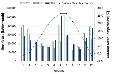
In this thesis, the electricity consumption for 3 years which had been observed in real time at 41 station points from Jan. 2012 to Dec. 2014 except for gas was used. The information related to outdoor temperature was compared with the average outdoor temperature for 3 years and the monthly electricity consumption for each year as shown in Fig. 3. by using the statistical climate data for Daejeon Metropolitan region provided by the Korea Meteorological Administration. If the monthly electricity consumptions are analyzed, it was found that the electricity consumptions during July and August were the highest except for 2013. Although the average temperatures in outdoor air for 3 years were similar during that period, it appeared that the deviations between the energy consumptions during summer of each year (June~August) were very big. Therefore, it is necessary to preferentially audit the problems related to the cooling energy consumption during a summer in the target building.
It is necessary to find out the points to be improved from the operation aspect by analyzing the specific energy consumption patterns using a simple regression analysis method and by calibrating the malfunctions of a used device and by adjusting the schedules, etc.
In order to show the energy performance profiles of G-building by using a simple regression analysis method, the independent and dependent variables must be selected first. Although there exist various kinds of variables such as the outdoor air temperatures, the number of occupants and the number of heating devices in an office, etc., when the dependent variables are selected, since it is hard to grasp the then real-time information on indoor temperatures of many buildings that were selected for green remodeling, the energy performance of a target building must be comprehended by proving the correlation with the outdoor temperatures based on the electricity consumption values using the monthly electricity bills obtained from the target buildings.
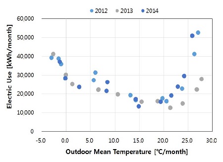
Thus, in this thesis, the independent variables are used as the average monthly outdoor temperature (X-Axis) and the dependent ones are used as the 3-year power consumption (Y-Axis) as shown in Fig. 4.
If the energy consumption patterns which are formed in the buildings for 3 years as shown in Fig. 4 are comprehended, the balance point temperature as the temperature at which cooling and heating are started must be set in order to analyze the energy performances by classifying the period into cooling, heating and non-cooling/heating periods.
In this thesis, the cooling & heating sections were adjusted while changing the temperature scale by 1℃ while using a trial and error method after deciding the scale of the outdoor temperature at 6℃ as the difference between the temperatures at which cooling (26℃) and heating(20℃) are started. At this time, the coefficient of determination(R2) is deducted from the trend lines of cooling and heating which were calculated by using the least square method. This means that there is a perfect correlation if R2 is 1 and there is no correlation if R2 is 0. In ASHRAE Fundamental 2013, it is recommended to use a value of R2 bigger than 0.75 since it is considered that the value is significant. Therefore, in this thesis, only a value bigger than 0.75 is allowed as the coefficient of determination. But in case that a value is smaller than 0.75, it is assumed that some points to be improved must be found out through some detailed audits.
The cases that a positive (+) slope appears in the heating section or a negative (-) slope does in the cooling one were excluded in order to obtain the balance-point temperature and the biggest value among the sums of the coefficients of determination for cooling and heating was selected. (But, the coefficient of determination for the non-cooling/heating section was not considered.)
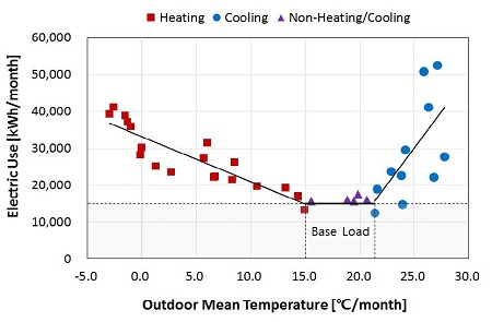
The prediction equations for temperature zones of the cooling, heating and non-cooling/heating sections were deducted by such a trial and error method like the Table 4 while using the method mentioned above. Although it was found that the coefficients of determination for heating area were less than or not more than 0.75 overall, it can be said that those for the cooling area were not. Therefore, the temperature sections, 14℃(for heating) and 21℃ (for cooling) whose sums of the determination coefficients for cooling and heating were highest among the temperature zones in Table 4 were set as the balance point temperatures. Accordingly, the temperature scope of the non-cooling/heating section (Intermediate Period) was decided as 15℃~20℃.
Fig 5. shows the energy performance profiles of the target buildings depending on the results which were deducted above. It can be found that the heating section (R2=0.8148) generally tends to relatively come close to the regression line, on the other hand, in the cooling section (R2=0.4176), the distribution of the energy consumptions is scattered on the basis of the regression line. Thus, it is necessary to improve the problems after finding out them by implementing the detailed audits for the cooling devices the determination coefficient for the cooling section is bigger than 0.75 at least.
3.3. Audit for Cooling Devices
As the results from an analysis of the electricity energy consumption which were obtained from each station point during the relevant period in order to audit the energy performance for cooling area, it was found that the energy consumption of the central plant equipment took the highest share as 26.8% among the total energy consumption as shown in Table 6. Especially, it was found that the energy consumption values the outdoor units (EHPs) which are located in the east and west were higher than the energy consumption values of two chillers. Therefore, in this thesis, the audits for the EHPs in the east and west were implemented preferentially and an additional audit for the day chillers whose energy consumption ratios are high was implemented.
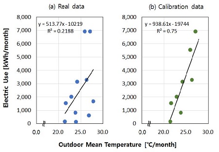
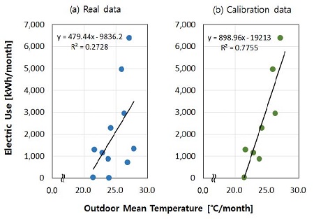
In case of the outdoor units(EHP) located in the east, while working together with AHU-2, they work as the heating sources for air conditioning of the offices on the first to fifth basements which are located in the north, east and south taking the highest energy consumption ratios during the cooling period. As the result from a simple regression analysis for the measured electricity consumption during the relevant period compared to the outdoor temperature, like Fig. 6, the determination coefficient for the outdoor unit (EHP) in the east 0.2188, so it is far lower than 0.75. It was found that the biggest reason was because the operator didn't cool the outdoor unit forcibly even though the outdoor temperature was very high at that time based on the government policy in 2013. In addition, it was shown that the energy consumption in July, 2014 was exceptionally higher than the other years as shown in Fig. 3 of Chapter 3. And it was found that too much cooling compared to usual years regardless of the government directions by the request of the pregnant occupant was represented in Fig. 6. Since the special data which was obtained from an audit mentioned above is somewhat inadequate for predicting the future energy consumption, the energy consumption data in July 2014 when the energy use was excessive due to the pregnant women's occupancy during the period June to September in 2013 was adjusted to the level, R2=0.75 by using a trial and error method and as the result, the value was calibrated like (b) of Fig. 6.
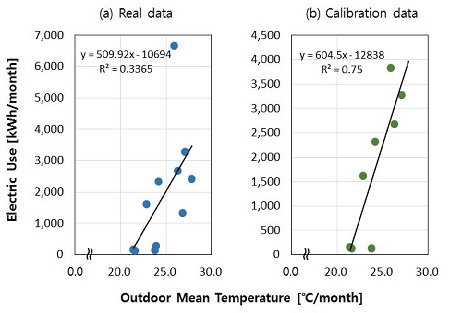
In case of the outdoor unit (EHP) in the west as the heat source for AHU-1 which air conditions in the south and the west of the first to fifth basements, it was found that the determination coefficient for this device was much lower than 0.75 like Fig. 7. (a) due to the same reason as the outdoor unit in the east considered the energy consumption pattern. In this case, it was found that the value corresponds to ASHRAE criteria only by excluding the data during June to August when the unit was abnormally operated by using a trial & error method. (Fig. 7. (b))
In case of the day chiller, as the result from the method mentioned above, it showed the same result as Fig 8. And as the result that the data for 2013 was excluded from the measurement value (a) and the consumption in July 2014 was calibrated to the level, 0.75, a prediction model was deducted like (b) of Fig 8.
3.4. Calibration and Prediction of Energy Consumption Values through an Audit
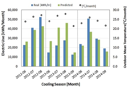
As the result from supplementing the energy consumption values of 3 units by substituting with the outdoor temperatures during the same period in order to compare the part of the energy consumption during the cooling period which was not comprehended correctly due to some abnormal use with the real measurement values by using the prediction model which was obtained by auditing the energy consumption values of such three units, the results as shown in Fig 9 were shown.
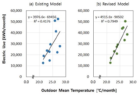
Comparison between existing and revised model after adapted calibrated values derived from three heat source equipments
Compared the determination coefficient during the existing cooling period, 0.4716, it was found that the model which was calibrated through an audit showed a closer correlation (R2=0.7949) with the outdoor temperature.
This means that the building can be operated at around 80% of correlation with the outdoor temperature only by improving the problems to the operation of the outdoor units (east & west) and the day chiller whose energy consumptions were high when the energy performance of the target building was audited by a simple regression analysis. In addition, as the result from comparing the real measurement value and the revised energy consumption value, the results were shown in Fig 10. The total electricity consumption which was measured for 3 years from 2012 to 2014 was 316,439kWh and the calibrated value was 340,047kWh. So, the calibrated model used more energy by around 23,608kWh compared with that of the existing model. However, the reason was because the forcibly reduced energy consumption was represented even though the energy consumption in 2013 got higher than usual temperatures. It was found that the consumption can be used somewhat less compared to the existing consumption if the revised model is operated during the same cooling period except for special cases. And in case of operating like that, the peak demand is reduced lower than the real measurement data, it was analyzed the total energy consumption can be reduced corresponding to the peak demand.
4. Conclusion
In case of enhancing the energy performance of the existing building, it has a weakness that it is somewhat difficult to obtain some specific information on the target building. In addition, any domestic audit guidelines have not suggested unlike the foreign countries and also it is in the situation that the methods using simulations while spending much time and cost are applied in most of studies and real cases. However, this study focused on the improvement of the energy performance of the existing building by auditing the energy consumption patterns and performances and finding out the problems of the target building while analyzing the correlation with the outdoor temperature based on the monthly consumption data by using a relatively simple linear regression analysis method. Although such a method is somewhat less accurate than the other methods, it was found that the energy performance and the problems can be comprehended only with some simple information on the energy consumption and the outdoor temperature. It was analyzed that such data can be used as the basic data when establishing the domestic green remodeling guidelines, especially, when establishing the energy performance audit method. However, it is somewhat restricted to apply the method to the general buildings since the target building for this study is one which a metering system is applied as a special case. Especially, since the accuracy can be enhanced when being considered the insulation and other heating load factors including the indoor temperature rather than the effect of the outdoor temperature especially in case of an office building, it is necessary to analyze the effects by using an analysis method like a multiple regression analysis method in a future study.
Acknowledgments
“This work was supported by the National Research Foundation of Korea(NRF) grant funded by the Korea government(MSIP) (No. 2011-0028075).”
References
- The report material of MOLIT(Ministry of Land, Infrastructure and Transport) in Korea, (2014, Dec, 30).
-
김승남, “건축물 유형별 에너지 소비 특성 분석과 활용”, 건축도시공간 연구소, (86), (2014, Apr).
Seung-Nam Kim, “Use and analysis of the energy consumption features depending on building type”, journal of AURI, (86), (2014, April). - Pacific Northwest National Liboratory and PECI, DOE(U.S. Department of Energy), “Advanced Energy Retrofit Guides, Office Buildings”, (2011, Sep).
- ASHRAE, 2011 ASHRAE Handbook-HVAC Applications, Energy Use And Management.
- ASHRAE, 2013 ASHRAE Fundamentals, Energy Estimating And Modeling Methods.
-
권경우, 회귀분석을 이용한 리모델링 건축물의 에너지 성능개선 분석 사례, 한국건축친환경설비학회, 9(1), (2015, Jan).
Kyungwoo Kwon, “A study on the cases for improving the remodeling building energy performance using the regression analysis”, journal of KIAEBS, 9(1), (2015, Jan). -
한혜심, 온열환경 지표를 활용한 사무소 건물의 에너지 효율화 방안 연구, 충남대학교 박사논문, p53, (2013, Oct).
Hyesim Han, “Methods for energy efficiency based on thermal comfprt fatprs in office building”, Ph.D Dissertation, Chungnam National University, p53, (2013, Sep). -
곽영훈, 실시간 건물 에너지 시뮬레이션 프레임워크 개발을 통한 냉방 시스템 예측 제어, 서울시립대학교 박사논문, p77-90, (2013, Dec).
Younghoon Kwak, “Predictive Control of Cooling System through the Development of Real-time Building Energy Simulation Framework”, Ph.D Dissertation, University of Seoul, p77-90, (2013, Dec). -
이승복, 회귀분석에 의한 건물에너지 사용량 예측기법에 관한 연구, 설비공학회 논문집, 12(12), (2000, Oct).
Seung-Bok Leigh, “A study for Predicting Building Energy Use with Regression Analysis”, (2000, Oct).

