A benchmark methodology to assess the energy performance of train station complexes
ⓒ 2019 KIEAE Journal
Abstract
A Train Station Complex (TSC) is a core facility in railway systems that have been preferred as public and mass transportation systems due to several advantages including safety, punctuality, and energy efficiency. Because of inherent building complexity, however, the energy performance model for TSC corresponding to periodical demands has not been developed yet. This study proposes an improved energy benchmark model that utilizes the regression coefficients of building performance parameters and normalization processes based on both measured and simulated data.
A multiple regression model is proposed for energy use intensity benchmarking of TSCs using measured and simulated energy consumption data. The model utilizes the analysis of variance to find effective factors in building performance evaluation and space programming for an early stage in building design.
By adjusting and refining the energy use intensity, the model proposes the conclusion that two existing TSCs are being operated more efficiently than theoretical results by 1.3% and 2.0%, respectively. By comparison of impact factors, the energy use intensity benchmark model was tested for its effectiveness of evaluating the energy performance of TSCs and optimizing space programs.
Keywords:
Train Station Complex, Energy Performance Assessment, Benchmark Methodology키워드:
복합철도역사, 에너지 성능 평가, 벤치마크 방법론1. Introduction
1.1. Train systems
Since the advent of Oystermouth Railway in the United Kingdom at the early 18th century, train systems have rapidly developed and extended to connect industrial, commercial, and residential areas[1]. As industrialization and modernization has progressed, train systems not only perform their main purpose of freight transportation, but they also become the center of the market system. Currently, train stations consist of additional facilities such as restaurants, offices, and malls, making the building consume a large amount of energy. In 2009, the rail-mode urban service averaged 63% more energy efficient than diesel and trolley bus systems[2, 3]. The 2014 Public Transportation Fact Book claims passenger trips by rail system (commuter and heavy rail) cover around 40% of the total number of passengers and over 50% of the total distance of passengers’ trips, and trains consumed about 20% of the diesel fuel that bus systems consumed[2, 3]. In Turkish transportation sector, train system was about 48% more efficient than diesel bus and truck systems[4].
A train station is one of the most important factors for successful train systems. Due to their size and operational characteristics, train stations typically consume great amount of energy. According to U.S. Department of Energy (US DOE) survey reports, buildings in the U.S. accounted for about 41% of total energy consumption in 2010 and about 74% of total electricity consumption[5]. This amount has increased by about 200% with respect to 1980’s levels. The building sector consumed $302 billion worth of electricity representing 82% of total energy expenditures[6]. Among the buildings, commercial buildings accounted for about 46% of total energy consumption[7]. Moreover, huge demands from the transport industry, including passenger, freight, and tourism, have made train stations to become transformed and designed as Train Station Complexes (TSCs). For instance, all of the stations for the Korean Train eXpress (KTX) service launched in 2004 by the Korea Railroad Corporation (KORAIL) were designed as TSCs to satisfy periodic demands in South Korea.
Typically, several studies dealing with transportation systems focused on the policy of greenhouse gas emission. Some dynamics for reduction of energy consumption focused on thermal transfer of vehicles envelope, speed control, and civil tunnel structure. Through the projection of interaction between greenhouse gas and climate conditions, the profit of electric train system was emphasized. To define energy consumption level of public transportation, advanced algorithm such as artificial neural network was tested and fuel types were analyzed[8, 9, 10].
Among the transportation systems, to reduce the overall energy consumption in train, a holistic approach utilized. There was an overview of available technologies for heating systems, time table optimization, and management of braking energy in train. By visualization of inter connection data in railway systems, energy saving method was proposed. Updated model of energy consumption for high speed train is proposed based on experimental data. To satisfy passenger’s demands while minimizing energy consumption, another effort for analysis of specific buildings was made in train. In addition, building energy saving design technologies and utilization of solar energy was made in train[11, 12, 13].
Many models predicting energy performance apply to complicated building complexes. A statistical machine learning framework was used to analyze the effect of input variables such as relative compactness, surface area, wall area, roof area, overall height, and orientation of residential buildings. The Gaussian mixture regression for modeling was used to quantify building energy use with parameterized and locally adaptive uncertainty and real time building simulation method. A Gaussian process and 2-stage Data Envelopment Analysis (DEA) model to determine energy savings and uncertainty levels in measurement were studied. DEA model was used to define total cost efficiency between road and rail transportation system. Additionally, depending on the building type, energy saving design method was presented[14, 16]. Despite the plentitude of energy performance models for commercial buildings, however, there is has been no model developed for energy performance evaluation of train stations[16, 17].
1.2. Problem statement
Even with the growing prevalence of TSCs, energy-performance metrics for energy policies have not been proposed in many studies. Because of operational characteristics, there are complexities and difficulties inherent to measuring accurate energy performance levels. Simple measurements of energy consumption and average EUI without consideration of impact factors and statistical validation can cause errors or imprecision in performance analysis.
This paper proposes a multiple regression model for EUI benchmarking of TSCs using the CBECS data and simulated energy consumption data. The model is tested to for effectiveness for building performance evaluation and space program design rule for energy policy. Section 2 discusses the basics of EUI indicator and benchmark tool, describes the choice of significant factors, and proposes the formulation of a multiple regression model. Using the data, the proposed model is tested in Section 3. Finally, the model is validated for its effectiveness of evaluating the energy performance of TSCs in Sections 4 and 5.
2. Methodology
2.1. EUI benchmark
Researchers have developed a method for detecting precise Energy Use Intensity (EUI: kWh/m2-yr or kBtu/sf-yr) levels of buildings: they commonly suggest using a simple regression model as the baseline for a benchmark. An equation of the model is given as
| (Eq. 1) |
where “α” is an intercept; “b1,⋯,bk” are regression coefficients; “χ1*,⋯χk*” are significant standardized factors;“ε” is random error[18, 19, 20, 21].
If the mean EUI of certain building types (intercept α) is defined, regression coefficients of factors (b1,⋯,bk),and standardized values of factors (χ1*,⋯χk*), the EUI of existing or future buildings can be evaluated.
Previous studies used the simple mean as the intercept “α” without reflecting normalized effects of each factor. The simple mean of EUI as an intercept “α” may cause statistical errors due to some outliers or unstandardized conditions. A modified equation is derived from (Eq. 1), one that lets the measured (observed) EUI be the EUI0, and the intercept “α” be the EUInorm. They then transform the equation as follows.
| (Eq. 2) |
where, EUI0 is measured EUI; b1,⋯,bk are regression coefficients; and χ1*,⋯χk* are standardized factors[22].
2.2. Share of floor spaces
TSCs consist of multiple building types in one structure, such as offices, retail, food service, cinema, and support areas. Among KORAIL TSCs in South Korea, the Hanhwa Yeoksa Corporation provided space programs. The company’s TSCs in Seoul consisted of office, mall, retail, food service, cinema, and indoor parking Area[23].
The CBECS report and the AIA guide categorized major commercial buildings as 14 different building types: education, food sales, food service, health care, lodging, retail, office, public assembly, public order & safety, religious worship, service, warehouse and storage, other, and vacant[24].
As compared to the space program, the CBECS report or the AIA guide do not specifically categorize cinema and indoor parking areas as major building types. Architecture 2030 analyzed the CBECS report in detail and found that entertainment, cultural, library, recreation, and social areas were included as public assembly spaces[25]. Indoor-parking areas typically do not have a specific heating and cooling system except minimum lighting and ventilation, so the category storage (self-storage) in Table 1. defines building types using the CBECS and Hanhwa Yeoksa data.
Office and mall areas cover about 70% of total floor space. Retail and food service areas are only 8.8% of total floor area, yet cover a large portion of operating income and may entice people to use the train system. The cinema covers 3.3% of a TSC’s total floor area. In terms of operational aspects, these four areas should be expanded and strengthened, and energy benchmarks for these zones should be emphasized.
2.3. Benchmark model
For clarity, the simple regression model is rewritten from (Eq. 2). The method used in this initial step was reported[26].
| (Eq. 3) |
However, this simple regression model is utilized to define single building type only. For this paper, the shares of floor space analyzed are added to the model as weighted values. As indicated in Table 1., the shares of space of office, enclosed mall, retail, food service, public assembly, and storage are 14.4% (0.144), 54.7% (0.547), 4.4% (0.044), 4.4% (0.044), 3.3% (0.033), and 18.6% (0.186) respectively. [IMPACTS in TSC] is obtained.
| (Eq. 4) |
By using the result, EUInorm of (Eq. 4) is rewritten as an adjusted multiple regression model for adjusted EUInorm reflecting the share of floor space.
| (Eq. 5) |
where EUI0 is the measured EUI, IMPACTS is the sum of each regression coefficient multiplied by standardized value.
2.4. Factors
Factors as explanatory variables from CBECS and EnergyPlus simulation were standardized to remove the effect of deviance out of each different scale.
| (Eq. 6) |
where, X is a value of the variable, μ is mean, and σ is standard deviation.
The standardized values of all variables (on X axis) and their EUIs (on Y axis) generated the data sets of table sandscatter plots. Then Regression Coefficient (RC) statistical Significance (Sig) as p-value was derived from one-way ANOVA test. The Sig (p-value) less than 0.05 have strong relationship between EUI (dependent variable) and factors (explanatory variable). Factors which have strong relation to changes in EUI are selected.
2.5. Analysis of measured data
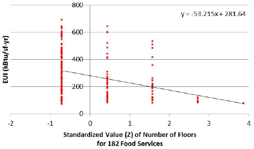
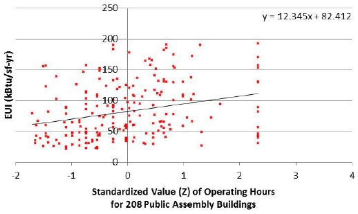
The CBECS report consists of several factors. Among them, 6 influential factors were chosen: building area (Area), building’s age (Age), number of floor (Floor), number of thermal zone (TZ), hour, heating degree days (HDD), cooling degree days (CDD), and HDD+CDD. Fig. 1. and 2. describe two examples out of 48 datasets: changes in EUI as changes in number of floors for 182 food service buildings, and changes in EUI as changes in operating hours for 208 public assembly buildings. Parts of results in Table 2. were reported[26].
Fig. 1. and 2. shows that the relations between EUI and factors were not clearly defined even if the slopes were displayed. Some values of R2 were too small to define relationship, which was caused by the some outliers out of large samples or the wide range of variances of data points. For the problems, one-way ANOVA test was used. Table 2. shows the results of RCs and Sigs from the test, and 15 factors are bolded.
In the building type of office, EUIs are increasing as operating hours, HDD, and HDD+CDD are increasing. In terms of climate condition, the changes in EUI of office may sensitive to HDD which can reflect heating required. However, enclosed mall, food service, public assembly, and storage buildings are relatively not sensitive to climate condition.
As indicated in Table 2., RC values of food service show the different patterns as compared to other building types. This result may be caused by the characteristics of food service building such as specific equipment (stove, oven, washer, fan, and large capacity freezer) and business model. All factors of enclosed mall and storage building do not have relations to changes in EUI, so these are neglected in finalizing multiple regression model.
2.6. Analysis of simulation results
Table 3. shows the conditions and template used for 90 simulations in EnergyPlus and OpenStudio.
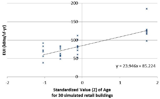
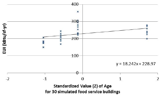
From the 90 simulated results, 21 datasets of all factors were generated. Fig. 3. and 4. show two examples out of the 21 datasets.
As indicated in Table 4., most results show similar results to CBECS, and some significant factors are confirmed. However, two highlighted factors as RCs of age in retail and food service show opposite trends of CBECS results. Two factors in the analysis of CBECS are removed in multiple regression model in this paper. In general, old building may consume more energy than new building due to performance of infiltration and penetration, which are strengthened by simulation results.
3. Result
3.1. Multiple regression model
From Table 2. and 4., all RCs and Sigs of factors were defined: Hour, HDD, and HDD+CDD for office; none of enclosed mall; Area, Age, Hour, and HDD+CDD for retail; Area, Age, Floor, and Hour for food service; Area, Age, TZ, and Hour for public assembly. With the factors, [IMPACTS of office] is obtained.
| (Eq. 7) |
where, R(X) is the regression coefficient of X, and Z(Y) is the standardized value of Y. Likewise, [IMPACTS of retail, food service, and public assembly] are obtained. From the equations, the adjusted multiple regression model for adjusted EUInorm is obtained.
| (Eq. 8) |
3.2. Case studies
Information of geometries and climate are as follows:
(a) Name: Seoul Station
(b) Climate conditions
- Location: Seoul, South Korea
- HDD: 2,431.8
- CDD: 881.2
(c) Building age: 12
(d) Total floor area: 95,168.9 m2
(e) Number of floors: 7
(f) Measured EUI: 249.4 kWh/m2-yr
(g) Floor area / Number of TZs
- Office: 13,704.3 m2 / 10
- Enclosed Mall: 52,057.4 m2 / 20
- Retail: 4,187.4 m2 / 20
- Food Service: 4,187.4 m2 / 20
- Cinema: 3,140.6 m2 / 5
- Parking: 17,891.8 m2 / 1
(h) Annual Operating Hours
- Office: 6,935
- Enclosed Mall: 4,380
- Retail: 4,380
- Food Service: 5,110
- Cinema: 4,380
- Parking: 6,935
From the values, the adjusted EUInorm is obtained:
| (Eq. 9) |
Architectural and climate information defined are as follows:
(a) Name: Cheongnyangni Station at Seoul
(b) Climate conditions
Location: Seoul, South Korea
- HDD: 2,431.8
- CDD: 881.2
(c) Building age: 5
(d) Total floor area: 177,787.4 m2
(e) Number of floors: 12
(f) Measured EUI: 207.5 kWh/m2-yr
(g) Floor area / Number of TZs
- Office: 20.842.4 m2 / 10
- Enclosed Mall: 92,423.8 m2 / 20
- Retail: 4,234.5 m2 / 20
- Food Service: 4,234.6 m2 / 20
- Cinema: 8,482.4 m2 / 5
- Parking: 47,572.2 m2 / 1
(h) Annual Operating Hours
- Office: 6,935
- Enclosed Mall: 4,380
- Retail: 4,380
- Food Service: 5,110
- Cinema: 4,380
- Parking: 6,935
From the values, the result of adjusted EUInorm is obtained:
| (Eq. 10) |
4. Discussion
Table 5. describe values of adjusted EUInorm of cases 1 and 2 were 246.4 kWh/m2-yr and 203.4 kWh/m2-yr, respectively. The amounts are1.2% and 2.0% smaller than the measured EUIs. The mean adjusted EUInorm was 224.9 kWh/m2-yr and 1.6% smaller than the mean measured EUI. Two values of adjusted EUInorm were commonly smaller than the measured EUIs, which means that both TSCs were consuming more energy than optimum planning.
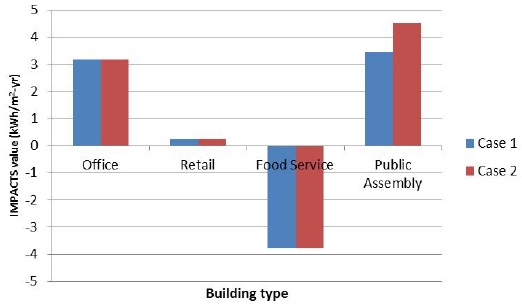
The results can be analyzed by the analysis of impact values of each building types. Fig. 5. indicates the weighted impact values (share of floor space multiplied by IMPACTS of building type) as building types in final multiple regression model. The values of office, retail, and public assembly were positive values, but the impact of food service was negative values.
For the public assembly, it can be seen that the pattern in energy consumption by area is rapidly increasing. However, the data in the case studies shows that the area differences in the cinema are much larger than the area differences, which may have caused the difference in energy use intensity in Fig. 5. Accordingly, office, retail, and public assembly increased EUI, so energy optimum design of three building types in TSCs could be required. As previously mentioned, it was confirmed that the impact of food service was quite large even though the share of floor area was relatively small. Large absolute values of RCs in food service could be a reason of changes in EUI. And also, three building types of office, retail, and public assembly were not designed energy efficiently, but food service buildings were relatively optimized to minimize impact on energy consumption. Because the impacts of three building types were larger than the impact of food service, two TSCs in Seoul were being operated inefficiently. For example as a space program design strategy, reducing operating hours for office or floor areas of public assembly can be more effective way for saving large amount of energy. It implies the fact that optimization of space program can contribute to building energy performance, and that architectural functionality can play a role to improve energy efficiency.
5. Conclusion
In this paper, the multiple regression model for TSCs’ energy performance benchmark is developed from the analysis of actual data and simulation results. The share of floor space determines the influence of each building type within the TSC. The analysis of datasets and scatter plots of factors defines the regression coefficients affecting building performance. Based on the shares and regression coefficients, the final model for adjusted EUInorm is obtained, and the results from the final model can be used to compare measured EUIs.
From the model, the mean values of adjusted EUInorm (224.9 kWh/m2-yr), obtained from the energy performance benchmark model can be utilized as a more precise baseline for TSCs. The advantage is that the final model can be a starting point when an insufficient amount of measured data is provided. Additionally, this model can be used to refine the other models without any normalization processes, as has been used in previous studies. Another advantage is that this model can intuitively assess and predict the energy consumption levels of existing and future TSCs, as well as define precise baseline data for other building types. Regarding the discussion, adjustment of share of floor space as building types contributes to improve energy efficiency of entire buildings. However, a follow-up study should be conducted to identify hidden relationships by sufficiently securing the number of samples used in the standardization process of the factors selected in the process.
Acknowledgments
This work was supported by the National Research Foundation of Korea (NRF) grant funded by the Korea government (MSIT) (No.2019R1G1A1006984).
References
- BBC. Mumbles railway was remarkable. BBC NEWS. [Online] March 25, 2007. [Cited: March 27, 2015.] http://news.bbc.co.uk, .
- J. Strickland, Energy Efficiency of different modes of transportation. Stanford: Stanford University Press, 2009.
- APTA. 2014 Public transportation fact book. Washington D.C. : APTA, 2014.
-
Z. Utlu and A. Hepbasli, Assessment of the energy utilization efficiency in the Turkish transportation sector between 2000 and 2020 using energy and exergy analysis method. 2006, Energy Policy, pp.1611-1618.
[https://doi.org/10.1016/j.enpol.2004.12.011]

- USDOE. Building Databook: Chapter 1. Building Sector. USDOE. [Online] 2015. [Cited: March 1, 2015.] http://buildingsdatabook.eren.doe.gov/ChapterIntro1.aspx, .
- USDOE. Building Databook: Chapter 6. Energy Supply. USDOE. [Online] 2015. [Cited: March 1, 2015.] http://buildingsdatabook.eren.doe.gov/ChapterIntro6.aspx, .
- USDOE. Building Databook: Chapter 3. Commercial Sector. USDOE. [Online] 2015. [Cited: March 1, 2015.] http://buildingsdatabook.eren.doe.gov/ChapterIntro2.aspx, .
-
A. Grahn and J. Hansson, Prospects for domestic biofuels for transport in Sweden 2030 based on current production and future plans. Wiley Interdisciplinary Reviews: Energy and Environment, 2014, pp.290-306.
[https://doi.org/10.1002/wene.138]

-
Y. Cheng, Y. Chang and L. Lu, Urban transportation energy and carbon dioxide emission reduction strategies. Applied Energy, 2015, pp.953-973.
[https://doi.org/10.1016/j.apenergy.2015.01.126]

-
J. DeCicco, The liquid carbon challenge: evolving views on transportation fuels and climate. Wiley Interdisciplinary Reviews: Energy and Environment, 2015, pp.98-114.
[https://doi.org/10.1002/wene.133]

-
A. Gonzalez-Gil, R. Palacin and P. Batty, Sustainable urban rail systems. Strategies and technologies for optimal management of regenerative braking energy. Energy Conversion and Management, 2013, pp.374-388.
[https://doi.org/10.1016/j.enconman.2013.06.039]

-
U. Brandes and D. Wagner, Using Graph Layout to Visualize Train Interconnection Data. Journal of Graph Algorithms and Applications, 2000, pp.135-155.
[https://doi.org/10.7155/jgaa.00028]

- R. Bosquet, et al. Model of High-Speed Train Energy Consumption. World Academy of Science, Engineering and Technology, 2013, pp.6-22.
-
S. Cho, et al, Methodology for energy strategy to prescreen the feasibility of Ground Source Heat Pump systems in residential and commercial buildings in the United States. Energy Strategy Reviews, Vol.18, 2017, pp.53-62.
[https://doi.org/10.1016/j.esr.2017.09.012]

-
J. Cho and Y. Kim, Analysis of Indoor Thermal Comfort and Energy Saving Based on Changes in the Office Building Envelope, Korea: Journal of KIEAE, Vol.18, No.2, 2018, pp.5-12.
[https://doi.org/10.12813/kieae.2018.18.2.005]

-
Y. Kim and H. Park, Typification and Models Related to Type and Attributes of Public Buildings, Korea: Journal of KIEAE, Vol.18, No.6, 2018, pp.69-81.
[https://doi.org/10.12813/kieae.2018.18.6.069]

-
E. Wanga, et al. Benchmarking energy performance of residential buildings using two-stage multifactor data envelopment analysis with degree-day based simple-normalization approach. Energy Conversion and Management, 2015, pp.530-542.
[https://doi.org/10.1016/j.enconman.2015.09.072]

- AIA. Integrating energy modeling in the design process. Washington D.C. : AIA, 2012.
- N. Nie, et al. Statistical Package for the Social Sciences. New York : McGraw-Hill, 1975.
-
J. Monts and M. Blissett, Assessing energy efficiency and energy conservation potential among commercial buildings: A statistical approach. Energy Vol.7, No.10, 1982, pp.861-869.
[https://doi.org/10.1016/0360-5442(82)90035-4]

- T. Sharp, Energy benchmarking in commercial office buildings. Washington D.C. : USDOE, 1996.
-
W. Chung, Y. Hui and Y. Lam, Benchmarking the energy efficiency of commercial buildings, Applied Energy, 2006, pp.1-13.
[https://doi.org/10.1016/j.apenergy.2004.11.003]

- Hanhwa. Seoul Station, Cheongnyangni Station. Hanhwa Yeoksa. [Online] 2015. [Cited: March 27, 2015.] http://www.hwsd.co.kr/, .
- USEIA. CBECS Table E2 Major Fuel Consumption Intensities by End Use for Non Mall. USEIA. [Online] 2008. [Cited: May 8, 2013.] http://www.eia.doe.gov/emeu/cbecs, .
- Architecture 2030, 2030 Challenge Targets: U.S. National Medians. Santa Fe, NM : 2030 Inc., 2012.
-
J. Ahn and S. Cho, Development of a statistical analysis model to benchmark the energy use intensity of subway stations. Applied Energy, Vol.179, 2016, pp.488-496.
[https://doi.org/10.1016/j.apenergy.2016.06.065]


